勾配法と誤差逆伝播法

誤差逆伝播法(back-propagation)

ニューラルネットワークモデル

この節では入力層，隠れ層，出力層からなる3層ニューラルネットワークを実装する．

using Base: @kwdef
using Parameters: @unpack # or using UnPack
using LinearAlgebra, Random, Statistics, PyPlot, ProgressMeter

@kwdef mutable struct NN{FT}
    n_batch::UInt32 # batch size
    n_in::UInt32 # number of input units
    n_hid::UInt32 # number of hidden units
    n_out::UInt32 # number of output units
    
    params::Dict{Any, Any} # weights and bias
    grads::Dict{Any, Any} = Dict() # gradient of params
end;

function NN(n_batch, n_in, n_hid, n_out)
    params = Dict()
    params["W1"] = 2(rand(n_in, n_hid) .- 0.5) / sqrt(n_in)
    params["W2"] = 2(rand(n_hid, n_out) .- 0.5) / sqrt(n_hid)
    params["b1"] = zeros(1, n_hid)
    params["b2"] = zeros(1, n_out)
    return NN{Float32}(n_batch=n_batch, n_in=n_in, n_hid=n_hid, n_out=n_out, params=params)
end;

mutable struct NNを用意し，重みの初期化(weight initialization) を行う同名の関数NNを用意する．重みの初期化の手法は複数ある(Glorot & Bengio, 2010)が，ここでは重みを\(w\)として，\(w \sim U\left(-1/\sqrt{n}, 1/\sqrt{n}\right)\)とする．ただし，\(n\)は入力ユニット数である．

Optimizerの作成

abstract typeとしてOptimizerタイプを作成する．

abstract type Optimizer
end

確率的勾配降下法(stochastic gradient descent; SGD) を実装する．

# SGD optimizer
@kwdef struct SGD{FT} <: Optimizer
    η::FT = 1e-2
end

function optimizer_update!(param, grad, optimizer::SGD)
    @unpack η = optimizer
    param[:, :] -= η * grad
end

optimizer_update! (generic function with 1 method)

次にAdam (Kingma & Ba, 2014) を実装する．

# Adam optimizer
@kwdef mutable struct Adam{FT} <: Optimizer
    α::FT  = 1e-4
    β1::FT = 0.9
    β2::FT = 0.999
    ϵ::FT = 1e-8
    ms = Dict()
    vs = Dict()
end

# Adam optimizer
function optimizer_update!(param, grad, optimizer::Adam)
    @unpack α, β1, β2, ϵ, ms, vs = optimizer
    key = objectid(param)
    if !haskey(ms, key) 
        ms[key], vs[key] = zeros(size(param)), zeros(size(param))
    end    
    m, v = ms[key], vs[key]
    m += (1 - β1) * (grad - m)
    v += (1 - β2) * (grad .* grad - v)
    param[:, :] -= α * m ./ (sqrt.(v) .+ ϵ)
end

optimizer_update! (generic function with 2 methods)

順伝播・逆伝播の実装

活性化関数を用意する．今回はsigmoid関数のみ使用する．

sigmoid(x) = 1 / (1 + exp(-x));
relu(x) = x .* (x .> 0);

\(f(\cdot)\)を活性化関数とする．順伝播(feedforward propagation)は以下のようになる．

\[\begin{split} \begin{align} \text{入力層 : }&\mathbf{z}^{(0)}=\mathbf{x}\\ \text{隠れ層 : }&\mathbf{z}^{(\ell)}=f\left(\mathbf{a}^{(\ell)}\right)\\ &\mathbf{a}^{(\ell+1)}=W^{(\ell+1)}\mathbf{z}^{(\ell)}+\mathbf{b}^{(\ell+1)}\\ \text{出力層 : }&\hat{\mathbf{y}}=\mathbf{z}^{(L)} \end{align} \end{split}\]

逆伝播(backward propagation)

\[\begin{split} \begin{align} \text{目的関数 : }&\mathcal{L}=\frac{1}{2}\left\|\hat{\mathbf{y}}-\mathbf{y}\right\|^{2}\\ \text{最急降下法 : }&\Delta W^{(\ell)}=-\eta \frac{\partial \mathcal{L}}{\partial W^{(\ell)}}\\ &\Delta \mathbf{b}^{(\ell)}=-\eta \frac{\partial \mathcal{L}}{\partial \mathbf{b}^{(\ell)}}\\ \text{誤差逆伝播法 : }&\frac{\partial \mathcal{L}}{\partial \hat{\mathbf{y}}}=\frac{\partial \mathcal{L}}{\partial \mathbf{z}^{(L)}}=\hat{\mathbf{y}}-\mathbf{y}\\ &\delta^{(L)}=\frac{\partial \mathcal{L}}{\partial \mathbf{z}^{(L)}} \frac{\partial \mathbf{z}^{(L)}}{\partial \mathbf{a}^{(L)}}=\left(\hat{\mathbf{y}}-\mathbf{y}\right) \odot f^{\prime}\left(\mathbf{a}^{(L)}\right)\\ &\mathbf{\delta}^{(\ell)}=\frac{\partial \mathcal{L}}{\partial \mathbf{z}^{(\ell)}} \frac{\partial \mathbf{z}^{(\ell)}}{\partial \mathbf{a}^{(\ell)}}=\left(W^{(\ell+1)}\right)^\top \delta^{(\ell+1)} \odot f^{\prime}\left(\mathbf{a}^{(\ell)}\right)\\ &\frac{\partial \mathcal{L}}{\partial W^{(\ell)}}=\frac{\partial \mathcal{L}}{\partial \mathbf{z}^{(\ell)}} \frac{\partial \mathbf{z}^{(\ell)}}{\partial \mathbf{a}^{(\ell)}} \frac{\partial \mathbf{a}^{(\ell)}}{\partial W^{(\ell)}}=\delta^{(\ell)}\left(\mathbf{z}^{(\ell-1)}\right)^\top\\ &\frac{\partial \mathcal{L}}{\partial \mathbf{b}^{(\ell)}}=\frac{\partial \mathcal{L}}{\partial \mathbf{z}^{(\ell)}} \frac{\partial \mathbf{z}^{(\ell)}}{\partial \mathbf{a}^{(\ell)}} \frac{\partial \mathbf{a}^{(\ell)}}{\partial \mathbf{b}^{(\ell)}}=\delta^{(\ell)} \end{align} \end{split}\]

バッチ処理を考慮すると，行列を乗ずる順番が変わる．

function update!(variable::NN, x::Array, y::Array, training::Bool, optimizer::Optimizer=SGD(), losstype::String="binary_crossentropy")
    @unpack n_batch, params, grads = variable 
    W1, W2, b1, b2 = params["W1"], params["W2"], params["b1"], params["b2"]
    
    # feedforward
    h = sigmoid.(x * W1 .+ b1) # hidden
    ŷ = sigmoid.(h * W2 .+ b2) # output
    error = ŷ - y
    
    if training # backward 
        if losstype == "binary_crossentropy"
            δ2 = error 
        elseif losstype == "squared_error"
            δ2 = error .* ŷ .* (1.0 .- ŷ)
        end
        δ1 = δ2 * W2' .* h .* (1.0 .- h)

        # get gradients
        grads["W1"] = x' * δ1
        grads["W2"] = h' * δ2
        grads["b1"] = sum(δ1, dims=1)
        grads["b2"] = sum(δ2, dims=1)

        # update params
        for key in keys(nn.params) 
            optimizer_update!(params[key], grads[key] / n_batch, optimizer)
        end
    end
    return error, ŷ, h
end

update! (generic function with 3 methods)

\[ \frac{d}{dx} \text{Sigmoid}(x) = \text{Sigmoid}(x) \cdot \left(1 - \text{Sigmoid}(x)\right) \]

であることに注意．

Zipser-Andersenモデル

Zipser-Andersenモデル [Zipser and Andersen, 1988] は頭頂葉の7a野のモデルであり，網膜座標系における物体の位置と眼球位置を入力として，頭部中心座標(head centered coordinate)に変換する．隠れ層はPPC(Posterior parietal cortex)の細胞のモデルになっている．

データセットの生成

物体位置の表現にはGaussian形式とmonotonic形式があるが，簡単のために，Gaussian形式を用いる．なお，monotonic形式については末尾の補足を参照してほしい．

# Gaussian 2d
function Gaussian2d(pos, sizex=8, sizey=8, σ=1)
    x, y = 0:sizex-1, 0:sizey-1
    X, Y = [i for i in x, j in 1:length(y)], [j for i in 1:length(x), j in y]
    x0, y0 = pos
    return exp.(-((X .- x0) .^2 + (Y .- y0) .^2) / 2σ^2)
end

Gaussian2d (generic function with 4 methods)

入力は64(網膜座標系での位置)+2(眼球位置信号)=66とする．眼球位置信号は原著ではmonotonic形式による32(=8ユニット×2(x, y方向)×2 (傾き正負))ユニットで構成されるが，簡単のために眼球位置信号も\(x, y\)の2次元とする．視覚刺激は-40度から40度までの範囲であり，10度で離散化する．よって，網膜座標系での位置は\(8\times 8\)の行列で表現される．位置は2次元のGaussianで表現する．ただし，1/e幅（ピークから1/eに減弱する幅）は15度である．\(1/e\)の代わりに\(1/2\)とすれば半値全幅(FWHM)となる．スポットサイズを\(w\)，Gaussianを\(G(x)\)とすると．\(G(x+w/2)=G/e\)より，\(\sigma=\frac{\sqrt{2}w}{4}\)と求まる．

# dataset parameter
θmax = 40.0 # degree, θ∈[-θmax, θmax]
Δθ = 10.0 # degree
stimuli_size = Int(2θmax / Δθ)
w = 15.0 # degree; 1/e width
σ = √2w/(4Δθ);

# training parameter
n_data = 10000
n_traindata = Int(n_data*0.95)
n_batch = 25 # batch size
n_iter_per_epoch = Int(n_traindata/n_batch)
n_epoch = 1000; # number of epoch

# generate positions
Random.seed!(0)
retinal_pos = (rand(n_data, 2) .- 0.5) * 2θmax # ∈ [-40, 40]
head_centered_pos = (rand(n_data, 2) .- 0.5) * 2θmax # ∈ [-40, 40]
eye_pos = head_centered_pos - retinal_pos; # ∈ [-80, 80]

# convert
input_retina = [hcat(Gaussian2d((retinal_pos[i, :] .+ θmax)/Δθ, stimuli_size, stimuli_size, σ)...) for i in 1:n_data];
input_retina = vcat(input_retina...)
eye_pos /= 2θmax;

# concat
x_data = hcat(input_retina, eye_pos) #_encoded)
y_data = vcat([hcat(Gaussian2d((head_centered_pos[i, :] .+ θmax)/Δθ, stimuli_size, stimuli_size, σ)...) for i in 1:n_data]...);

# split
x_traindata, y_traindata = x_data[1:n_traindata, :], y_data[1:n_traindata, :]
x_testdata, y_testdata = x_data[n_traindata+1:end, :], y_data[n_traindata+1:end, :];

モデルの定義を行う．

# model parameter
n_in = stimuli_size^2 + 2 # number of inputs
n_hid = 16   # number of hidden units
n_out = stimuli_size^2   # number of outputs
η = 1e-2  # learning rate
losstype = "binary_crossentropy" # "squared_error"

nn = NN(n_batch, n_in, n_hid, n_out);
optimizer = SGD(η=η); 
#optimizer = Adam();

学習を行う．

error_arr = zeros(Float32, n_epoch); # memory array of each epoch error

@showprogress "Training..." for e in 1:n_epoch
    for iter in 1:n_iter_per_epoch
        idx = (iter-1)*n_batch+1:iter*n_batch
        error, _, _ = update!(nn, x_traindata[idx, :], y_traindata[idx, :], true, optimizer, losstype)
        error_arr[e] += sum(error .^ 2)
    end 
    error_arr[e] /= n_traindata
end

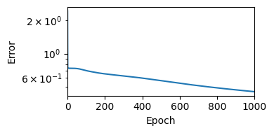
損失の変化を描画する．

figure(figsize=(4,2))
semilogy(error_arr)
ylabel("Error"); xlabel("Epoch"); xlim(0, n_epoch)
tight_layout()

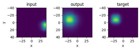
テストデータを用いて，出力を確認する．

x, y = x_testdata[1:2, :], y_testdata[1:2, :]
error, ŷ, h = update!(nn, x, y, false);

id = 1
figure(figsize=(6,2))
ax1 = subplot(1,3,1); title("input")
ax1.imshow(reshape(x[id, 1:64], (stimuli_size, stimuli_size))', interpolation="gaussian", extent=[-θmax, θmax, θmax, -θmax])
ax1.add_patch(plt.Circle((x[id, 65:66])*2θmax, radius=2, color="tab:red", fill=false))
xlabel("x"); ylabel("y");

ax2 = subplot(1,3,2); title("output")
ax2.imshow(reshape(ŷ[id, :], (stimuli_size, stimuli_size))', interpolation="gaussian", extent=[-θmax, θmax, θmax, -θmax])
ax2.add_patch(plt.Circle((x[id, 65:66])*2θmax, radius=2, color="tab:red", fill=false))
xlabel("x");

ax3 = subplot(1,3,3); title("target")
ax3.imshow(reshape(y[id, :], (stimuli_size, stimuli_size))', interpolation="gaussian", extent=[-θmax, θmax, θmax, -θmax])
ax3.add_patch(plt.Circle((x[id, 65:66])*2θmax, radius=2, color="tab:red", fill=false))
xlabel("x");

tight_layout()

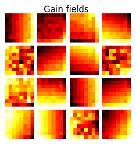
重みW1におけるゲインフィールドの描画を行う．

# Plot Gain fields
figure(figsize=(3.2, 3))
suptitle("Gain fields", fontsize=12)
subplots_adjust(hspace=0.1, wspace=0.1, top=0.925)
for i in 1:n_hid
    subplot(4, 4, i)
    imshow(reshape(nn.params["W1"][1:stimuli_size^2, i], (stimuli_size, stimuli_size)), cmap="hot")
    axis("off")
end

補足：Monotonic formatによる位置のエンコーディング

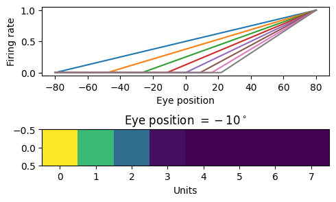
monotonic形式を入力の眼球位置と出力の頭部中心座標で用いるという仮定には，視覚刺激を中心窩で捉えた際，得られる眼球位置信号を頭部中心座標での位置の教師信号として使用できるという利点がある．(Andersen & Mountcastle, J. Neurosci. 1983)では Parietal visual neurons (PVNs)の活動を調べ，傾き正あるいは負．0度をピークとして減少あるいは上昇の4種類あることを示した．前者は一次関数（とReLU関数）で記述可能である．

get_line(p1, p2) = [(p2[2]-p1[2])/(p2[1]-p1[1]), (p2[1]*p1[2] - p1[1]*p2[2])/(p2[1]-p1[1])] # [slope, intercept]
eye_pos_coding(x; linear_param) = relu(linear_param[1, :] * x .+ linear_param[2, :])

x = -2θmax:1:2θmax
slope_param = hcat([get_line([80, 1], [-80, -2(i-1)/stimuli_size]) for i in 1:stimuli_size]...)
y = hcat(eye_pos_coding.(x; linear_param=slope_param)...)
eye_pos_encoded = eye_pos_coding(-10; linear_param=slope_param)

figure(figsize=(5,3))
subplot(2,1,1); plot(x, y'); xlabel("Eye position"); ylabel("Firing rate")
subplot(2,1,2); imshow(eye_pos_encoded[:, :]'); title(L"Eye position $=-10^\circ$"); xlabel("Units") 
tight_layout()

参考文献

ZA88

D Zipser and R A Andersen. A back-propagation programmed network that simulates response properties of a subset of posterior parietal neurons. Nature, 331(6158):679–684, February 1988.