格子細胞のデコーディング
Contents
格子細胞のデコーディング#
グリッド細胞(Grid Cells)#
空間基底としてのグリッド細胞#
海馬には場所特異的に発火する場所細胞(place cell)があり,これはO’keefeによって発見された.次にMay-Britt MoserとEdvard Moserが六角形格子状の場所受容野を持つグリッド細胞(格子細胞, grid cell)を内側嗅内皮質(medial entorhinal cortex; MEC)で発見した.この3人は2014年のノーベル生理学・医学賞を受賞している.
データについて#
格子細胞の活動データはMoser研が公開しており,https://www.ntnu.edu/kavli/research/grid-cell-dataからダウンロードできる.公開されているデータはMATLABのmatファイル形式である.使用するデータ:10704-07070407_POS.mat, 10704-07070407_T2C3.mat
これらのファイルはhttps://archive.norstore.no/pages/public/datasetDetail.jsf?id=8F6BE356-3277-475C-87B1-C7A977632DA7からダウンロードできるファイルの一部である.以下では./data/grid_cells_data/ディレクトリの下にファイルを置いている.
データの末尾の”POS”と”T2C3”の意味について説明しておく.まず,”POS”はpost, posx, posyを含む構造体でそれぞれ試行の経過時間,x座標, y座標である.座標は\([-50, 50]\)で記録されている.1m四方の正方形の部屋で,原点を部屋の中心としている.”T2C3”はtがtetrode(テトロード電極)でcがcell(細胞)を意味する.後ろの数字は番号付けである.
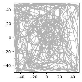
ラットの行動軌跡と発火の描画#
データを読み込む.
using PyPlot, MAT, StatsBase, FFTW
# from http://www.ntnu.edu/kavli/research/grid-cell-data
pos = matopen("../_static/datasets/grid_cells_data/10704-07070407_POS.mat")
spk = matopen("../_static/datasets/grid_cells_data/10704-07070407_T2C3.mat")
MAT.MAT_v5.Matlabv5File(IOStream(<file ../_static/datasets/grid_cells_data/10704-07070407_T2C3.mat>), false, #undef)
posファイル内の構造は次のようになっている.
pos["post"]: times at which positions were recordedpos["posx"]: x positionspos["posy"]: y positionsspk["cellTS"]: spike times
post = read(pos, "post")[:] #  times at which positions were recorded
posx = read(pos, "posx")[:] #x positions
posy = read(pos, "posy")[:] # y positions
spkt = read(spk, "cellTS")[:] #spike time

println(size(post), size(posx), size(posy), size(spkt))
(30000,)(30000,)(30000,)(2326,)
行動軌跡を描画する.
figure(figsize=(3,3))
plot(posx, posy, color="k", alpha=0.3)
xlim(-50, 50); ylim(-50, 50)
tight_layout()
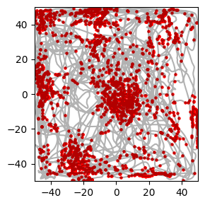
発火を描画するために発火時刻 spkt のそれぞれの要素と最も近い post のインデックスを求める関数を実装する.
function nearest_pos(array, value)
    idx = argmin(abs.(array .- value))
    return idx
end
nearest_pos (generic function with 1 method)
idx = [nearest_pos(post, t) for t in spkt]

print(size(idx))
(2326,)
figure(figsize=(3,3))
plot(posx, posy, color="k", alpha=0.3)
scatter(posx[idx], posy[idx], color="r", s=5)
xlim(-50, 50); ylim(-50, 50)
tight_layout()
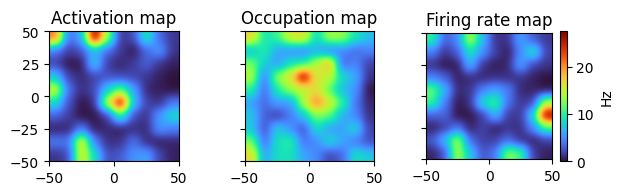
発火率マップ#
発火率\(\lambda(\boldsymbol{x})\)は,場所\(\boldsymbol{x}=(x,y)\)で記録されたスパイクの回数を,場所\(\boldsymbol{x}\)における滞在時間(s)で割ることで得られる.
ただし,\(n\)はスパイクの回数,\(T\)は計測時間,\(g(\cdot)\)はGaussain Kernel(中身の分子が平均,分母が標準偏差),\(\boldsymbol{s}_i\)は\(i\)番目のスパイクの発生した位置,\(\boldsymbol{y}(t)\)は時刻\(t\)でのラットの位置である.分母は積分になっているが,実際には離散的に記録をするので,累積和に変更し,\(dt\)を時間のステップ幅(今回は0.02s)とする.
この式の分母はマウスの位置,分子はニューロンが発火したときのマウスの位置についてそれぞれカーネル密度推定 (kernel density estimation)を行うことを意味する.今回はヒストグラムを求め,描画の際にGaussianで平滑化することで計算量を下げることとする.
発火数のヒストグラムを描画する.PyPlotでhist2D(posx[idx], posy[idx], bins=10, cmap="jet")などとする方が簡便だが,今回はhistgramの各binの値を用いるためにStatsBase.jlを用いる.
activ_hist = fit(Histogram, (posy[idx], posx[idx]), (-50:10:50, -50:10:50)).weights # activation
occup_hist = fit(Histogram, (posy, posx), (-50:10:50, -50:10:50)).weights # occup position while trajectory
occup_hist *= 0.02 # one time step is 0.02s
occup_hist[occup_hist .== 0] .= 1 # avoid devide by zero

rate_hist = activ_hist ./ occup_hist;
fig, ax = subplots(1, 3, figsize=(6.5, 2), sharex="all", sharey="all")
titles = ["Activation map", "Occupation map", "Firing rate map"]
hists = [activ_hist, occup_hist, rate_hist]
for (i, (t, h)) in enumerate(zip(titles, hists))
    ax[i].set_title(t)
    ims = ax[i].imshow(h, origin="lower", cmap="turbo", interpolation="gaussian", extent=[-50, 50, -50, 50])
    if i == 3
        fig.colorbar(ims, label="Hz", ax=ax[i])
    end
end
tight_layout()
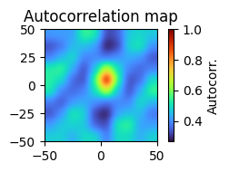
Autocorrelation Map#
2次元の自己相関マップ (autocorrelation map)を描画する.
function correlate_fft(x, y)
    corr = fftshift(real(ifft(fft(x) .* conj(fft(y)))))
    return corr / maximum(corr)
end;
corr_map = correlate_fft(rate_hist, rate_hist);
figure(figsize=(3, 2))
title("Autocorrelation map")
imshow(corr_map, origin="lower", cmap="turbo", interpolation="gaussian", extent=[-50, 50, -50, 50])
colorbar(label="Autocorr.")
tight_layout()