マルコフ連鎖モンテカルロ法 (MCMC)#

前節では解析的に事後分布の計算をした．事後分布を近似的に推論する方法の1つにマルコフ連鎖モンテカルロ法 (Markov chain Monte Carlo methods; MCMC) がある．他の近似推論の手法としてはLaplace近似や変分推論（variational inference）などがある．MCMCは他の手法に比して，事後分布の推論だけでなく，確率分布を神経活動で表現する方法を提供するという利点がある．

Note

変分推論は入れた方がいいと思うが，紙幅の都合上いれられるか微妙である．

データを\(X\)とし，パラメータを\(\theta\)とする．

\[ p(\theta\mid X)=\frac{p(X\mid \theta)p(\theta)}{\int p(X\mid \theta)p(\theta)d\theta} \]

分母の積分計算\(\int p(X\mid \theta)p(\theta)d\theta\)が求まればよい．

モンテカルロ法#

マルコフ連鎖#

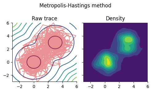
Metropolis-Hastings法#

using Base: @kwdef
using Parameters: @unpack
using PyPlot, LinearAlgebra, Random, Distributions, ForwardDiff, KernelDensity
rc("axes.spines", top=false, right=false)

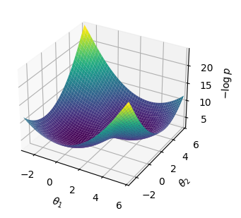
mixed_gauss = MixtureModel([MvNormal(zeros(2), I), MvNormal(3*ones(2), I)], [0.5, 0.5]) # 分布を混ぜる

MixtureModel{IsoNormal}(K = 2)
components[1] (prior = 0.5000): IsoNormal(
dim: 2
μ: [0.0, 0.0]
Σ: [1.0 0.0; 0.0 1.0]
)

components[2] (prior = 0.5000): IsoNormal(
dim: 2
μ: [3.0, 3.0]
Σ: [1.0 0.0; 0.0 1.0]
)

x = -3:0.1:6
pd(x₁, x₂) = logpdf(mixed_gauss, [x₁, x₂])

mixed_gauss_heat = pd.(x, x');

xpos = x * ones(size(x))'

fig = plt.figure(figsize=(4,3))
ax = fig.add_subplot(projection="3d")
surf = ax.plot_surface(xpos, xpos', -mixed_gauss_heat, cmap="viridis")
ax.set_xlim(-3, 6); ax.set_ylim(-3, 6); 
ax.set_xlabel(L"$\theta_1$"); ax.set_ylabel(L"$\theta_2$"); ax.set_zlabel(L"$-\log p$"); 
tight_layout()

# Metropolis-Hastings method; log_p: unnormalized log-posterior
function GaussianMH(log_p::Function, θ_init::Vector{Float64}, σ::Float64, num_iter::Int)
    d = length(θ_init)
    samples = zeros(d, num_iter)
    num_accepted = 0
    θ = θ_init # init position
    for m in 1:num_iter
        θ_ = rand(MvNormal(θ, σ*I))
        mH = log_p(θ) + logpdf(MvNormal(θ, σ*I), θ_)       # initial Hamiltonian
        mH_ = log_p(θ_) + logpdf(MvNormal(θ_, σ*I), θ)    # final Hamiltonian
        
        if min(1, exp(mH_ - mH)) > rand()
            θ = θ_ # accept
            num_accepted += 1
        end
        samples[:, m] = θ
    end
    return samples, num_accepted
end;

log_p(θ) = logpdf(mixed_gauss, θ);
grad(θ)= ForwardDiff.gradient(log_p, θ)

grad (generic function with 1 method)

θm, num_accepted = GaussianMH(log_p, [1.0,0.5], 1.0, 2000)

([1.0 0.5551053858555393 … 2.5978715364957816 2.5978715364957816; 0.5 -0.6019397439354577 … 2.2316937524389115 2.2316937524389115], 1191)

size(θm)

(2, 2000)

Um = kde((θm[1, :], θm[2, :]));

fig, ax = subplots(1, 2, figsize=(5, 3), sharex="all", sharey="all")
fig.suptitle("Metropolis-Hastings method")
ax[1].set_title("Raw trace")
ax[1].contour(x, x, -mixed_gauss_heat)
ax[1].plot(θm[1, :], θm[2, :], color="tab:red", alpha=0.5)
ax[1].set_xlim(-3,6); ax[1].set_ylim(-3,6)
ax[2].set_title("Density")
ax[2].contourf(Um.x, Um.x, Um.density)
fig.tight_layout()

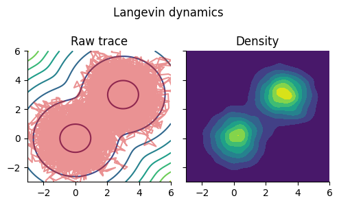
ランジュバン・モンテカルロ法 (LMC)#

http://watanabe-www.math.dis.titech.ac.jp/~kohashi/document/bayes_51.pdf

https://qiita.com/karadaharu/items/6c015ec99f30667808f2

https://en.wikipedia.org/wiki/Metropolis-adjusted_Langevin_algorithm

拡散過程

\[ {\frac{d\theta}{dt}}=\nabla \log p (\theta)+{\sqrt 2}{d{W}} \]

Euler–Maruyama法により，

β = 1
ρ = sqrt(2*ϵ);

nt = 10000
ϵ = 0.1

θl = zeros(nt, 2)
θ = [1.0,0.5]
for t in 1:nt
    θ += ϵ * β * grad(θ) + ρ * randn(2)
    θl[t, :] = θ
end

Ul = kde((θl[:, 1], θl[:, 2]));

fig, ax = subplots(1, 2, figsize=(5, 3), sharex="all", sharey="all")
fig.suptitle("Langevin dynamics")
ax[1].set_title("Raw trace")
ax[1].contour(x, x, -mixed_gauss_heat)
ax[1].plot(θl[:, 1], θl[:, 2], color="tab:red", alpha=0.5)
ax[1].set_xlim(-3,6); ax[1].set_ylim(-3,6)
ax[2].set_title("Density")
ax[2].contourf(Ul.x, Ul.x, Ul.density)
fig.tight_layout()

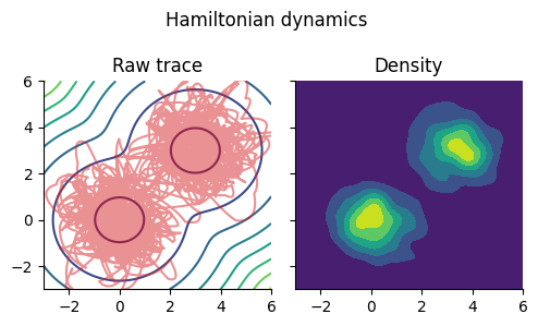
ハミルトニアン・モンテカルロ法 (HMC法)#

ハミルトニアン・モンテカルロ法(Hamiltonian Monte Calro)あるいはハイブリッド・モンテカルロ法(Hybrid Monte Calro)という

一般化座標を\(\mathbf{q}\), 一般化運動量を\(\mathbf{p}\)とする．ポテンシャルエネルギーを\(U(\mathbf{q})\)としたとき，古典力学（解析力学）において保存力のみが作用する場合のハミルトニアン (Hamiltonian) \(\mathcal{H}(\mathbf{q}, \mathbf{p})\)は

\[ \mathcal{H}(\mathbf{q}, \mathbf{p}):=U(\mathbf{q})+\frac{1}{2}\|\mathbf{p}\|^2 \]

となる．このとき，次の2つの方程式が成り立つ．

\[ \frac{d\mathbf{q}}{dt}=\frac{\partial \mathcal{H}}{\partial \mathbf{p}}=\mathbf{p},\quad\frac{d\mathbf{p}}{dt}=-\frac{\partial \mathcal{H}}{\partial \mathbf{q}}=-\frac{\partial U}{\partial \mathbf{q}} \]

これをハミルトンの運動方程式(hamilton’s equations of motion) あるいは正準方程式 (canonical equations) という．

この処理をMetropolis-Hastings法における採用・不採用アルゴリズムという．

リープフロッグ(leap frog)法により離散化する．

function leapfrog(grad::Function, θ::Vector{Float64}, p::Vector{Float64}, ϵ::Float64, L::Int)
    for l in 1:L
        p += 0.5 * ϵ * grad(θ)
        θ += ϵ * p
        p += 0.5 * ϵ * grad(θ)
    end
    return θ, p
end;

# Hamiltonian Monte Carlo method; log_p: unnormalized log-posterior
function HMC(log_p::Function, θ_init::Vector{Float64}, ϵ::Float64, L::Int, num_iter::Int)
    grad(θ)= ForwardDiff.gradient(log_p, θ)
    d = length(θ_init)
    samples = zeros(d, num_iter)
    num_accepted = 0
    θ = θ_init # init position
    for m in 1:num_iter
        p = randn(d) # get momentum        
        H = -log_p(θ) + 0.5 * p' * p        # initial Hamiltonian
        θ_, p_ = leapfrog(grad, θ, p, ϵ, L) # update
        H_ = -log_p(θ_) + 0.5 * p_' * p_    # final Hamiltonian
        
        if min(1, exp(H - H_)) > rand()
            θ = θ_ # accept
            num_accepted += 1
        end
        samples[:, m] = θ
    end
    return samples, num_accepted
end;

ps = zeros(nt, 2)
θs = zeros(nt, 2)
p = randn(2)
θ = randn(2)
for t in 1:nt
    if t in 20:10:nt
        p = randn(2)
    end
    p += 0.5 * ϵ * grad(θ)
    θ += ϵ * p
    p += 0.5 * ϵ * grad(θ)
    ps[t, :] = p
    θs[t, :] = θ
end

Us = kde((θs[:, 1], θs[:, 2]));

fig, ax = subplots(1, 2, figsize=(5, 3), sharex="all", sharey="all")
fig.suptitle("Hamiltonian dynamics")
ax[1].set_title("Raw trace")
ax[1].contour(x, x, -mixed_gauss_heat)
ax[1].plot(θs[:, 1], θs[:, 2], color="tab:red", alpha=0.5)
ax[1].set_xlim(-3,6); ax[1].set_ylim(-3,6)
ax[2].set_title("Density")
ax[2].contourf(Us.x, Us.x, Us.density)
fig.tight_layout()

ToDo: 自己相関確認する

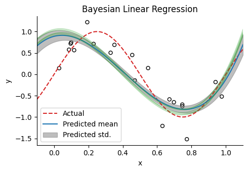
線形回帰への適応#

# Generate Toy datas
num_train, num_test = 20, 100 # sample size
dims = 4 # dimensions
σy = 0.3

polynomial_expansion(x; degree=3) = hcat([x .^ p for p in 0:degree]...);

Random.seed!(0);
x = rand(num_train)
y = sin.(2π*x) + σy * randn(num_train);
ϕ = polynomial_expansion(x, degree=dims-1) # design matrix

xtest = range(-0.1, 1.1, length=num_test)
ytest = sin.(2π*xtest)
ϕtest = polynomial_expansion(xtest, degree=dims-1);

log_joint(w, ϕ, y, σy, μ₀, Σ₀) = sum(logpdf.(Normal.(ϕ * w, σy), y)) + logpdf(MvNormal(μ₀, Σ₀), w);

α, β = 1e-3, 5.0

(0.001, 5.0)

w = randn(dims)
μ₀ = zeros(dims)
Σ₀ = 1/α * I;

ulp(w) = log_joint(w, ϕ, y, σy, μ₀, Σ₀)

ulp (generic function with 1 method)

w_init = rand(MvNormal(μ₀, Σ₀), 1)[:, 1]

4-element Vector{Float64}:
  11.502179436027728
 -29.136001309910146
 -28.331966074802352
   1.0557387545081587

@time samples, num_accepted = HMC(ulp, w_init, 1e-2, 10, 500)

  0.705381 seconds (4.15 M allocations: 234.361 MiB, 6.89% gc time, 95.22% compilation time)

([19.50061710033911 14.530099264391572 … 1.0224752923699738 1.055083645424437; -20.70857404957331 -19.669197492699 … 0.8438407654862355 0.9798655880237325; -21.20487540951859 -19.63123807655118 … -12.5972265388629 -12.627755360787681; 6.952173509808509 8.573602114577975 … 10.664214672362544 10.58188931372589], 499)

plot(samples[1, :])

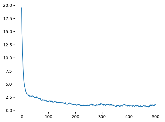
1-element Vector{PyCall.PyObject}:
 PyObject <matplotlib.lines.Line2D object at 0x000000011FF7E280>

yhmc = ϕtest * samples[:, 300:end];
yhmc_mean = mean(yhmc, dims=2)[:];
yhmc_std = std(yhmc, dims=2)[:];

figure(figsize=(5,3.5))
title("Bayesian Linear Regression")
scatter(x, y, facecolor="None", edgecolors="black", s=25) # samples
plot(xtest, ytest, "--", label="Actual", color="tab:red")  # regression line
plot(xtest, yhmc_mean, label="Predicted mean", color="tab:blue")  # regression line
fill_between(xtest, yhmc_mean+yhmc_std, yhmc_mean-yhmc_std, alpha=0.5, color="tab:gray", label="Predicted std.")
for i in 1:5
    plot(xtest, yhmc[:, end-i], alpha=0.3, color="tab:green")
end
xlabel("x"); ylabel("y"); legend()
xlim(-0.1, 1.1); tight_layout()

Juliaで学ぶ計算論的神経科学

マルコフ連鎖モンテカルロ法 (MCMC)

Contents